IV. Counterparty Credit Risk
I. Introduction
1. In March 2014, the Basel Committee on Banking Supervision (BCBS) published a new approach for measurement of counterparty credit risk exposure associated with OTC derivatives, exchange-traded derivatives, and long settlement transactions, the standardised approach for CCR (SA-CCR). The approach in the Central Bank’s Standards for CCR closely follows the SA-CCR as developed by the BCBS in all material areas of substance.
2. The BCBS developed the SA-CCR to replace the two previous non-internal model methods, the Current Exposure Method (CEM) and the Standardized Method (SM). The SA-CCR was designed to be more risk sensitive than CEM and SM. It accurately recognizes the effects of collateralization and recognizes a benefit from over-collateralization. It also provides incentives for centralized clearing of derivative transactions.
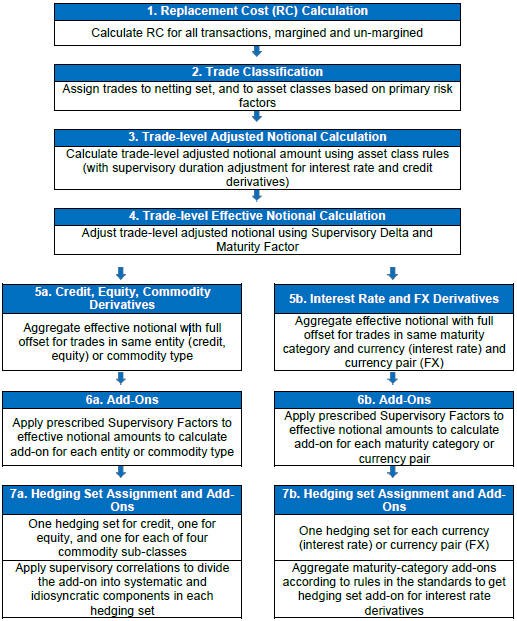
3. As is the case with the CEM, under the SA-CCR the exposure at default (EAD) is calculated as the sum of two components: (i) replacement cost (RC), which reflects the current value of the exposure adjusted for the effects of net collateral including thresholds, minimum transfer amounts, and independent amounts; and (ii) potential future exposure (PFE), which reflects the potential increase in exposure until the closure or replacement of the transactions. The PFE portion consists of a multiplier that accounts for over-collateralization, and an aggregate add-on derived from the summation of add-ons for each asset class (interest rate, foreign exchange, credit, equity, and commodity), which in turn are calculated at the hedging set level.
II. Clarifications
A. Replacement Cost
4. Note that in mathematical terms, replacement cost for un-margined transactions is calculated as:
RC = max(V − C; 0)
where RC is replacement cost, V is the total current market value of all derivative contracts in the netting set combined, and C is the net value of collateral for the netting set, after application of relevant haircuts. (In the CCR Standards, the quantity V-C is referred to as the Net Current Value, or NCV.)
5. For margined transactions, the calculation becomes:
RC = max(V − C; TH + MTA − NICA; 0)
where TH is the threshold level of variation that would require a transfer of collateral, MTA is the minimum transfer amount of the collateral, and NICA is the Net Independent Collateral Amount equal to the difference between the value of any independent collateral posted by a counterparty and any independent collateral posted by the bank for that counterparty, excluding any collateral that the bank has posted to a segregated, bankruptcy remote account.
6.When determining the RC component of a netting set, the netting contract must not contain any clause which, in the event of default of a counterparty, permits a non-defaulting counterparty to make limited payments only, or no payments at all, to the estate of the defaulting party, even if the defaulting party is a net creditor.
B. Netting
7. The Standards requires that a bank should apply netting only when it can satisfy the Central Bank that netting is appropriate, according to the specific requirements established in the Standards . Banks should recognize that this requirement would likely be difficult to meet in the case of trades conducted in jurisdictions lacking clear legal recognition of netting, which at present is the case in the UAE.
8. If netting is not recognized, then netting sets still should be used for the calculation. However, since each netting set must contain only trades that can be netted, each netting set is likely to consist of a single transaction. The calculations of EAD can still be performed, although they simplify considerably.
9. Note that there may be more than one netting set for a given counterparty. In that case, the CCR calculations should be performed for each netting set individually. The individual netting set calculations can be aggregated to the counterparty level for reporting or other purposes.
C. PFE Multiplier
10. For the multiplier of the PFE component, when the collateral held is less than the net market value of the derivative contracts (“under-collateralization”), the current replacement cost is positive and the multiplier is equal to one (i.e. the PFE component is equal to the full value of the aggregate add-on). Where the collateral held is greater than the net market value of the derivative contracts (“over-collateralization”), the current replacement cost is zero and the multiplier is less than one (i.e. the PFE component is less than the full value of the aggregate add-on).
D. Supervisory Duration
11. The Supervisory Duration calculation required in the Standards is in effect the present value of a continuous-time annuity of unit nominal value, discounted at a rate of 5%. The implied annuity is received between dates S and E (the start date and the end date, respectively), and the present value is taken to the current date.
12. For interest rate and credit derivatives, the supervisory measure of duration depends on each transaction’s start date S and end date E. The following Table presents example transactions and illustrates the values of S and E, expressed in years, which would be associated with each transaction, together with the maturity M of the transaction.
Instrument M S E Interest rate or credit default swap maturing in 10 years 10 0 10 10-year interest rate swap, forward starting in 3 years 13 3 13 Forward rate agreement for time period starting in 125 days and ending in one year 1 0.5 1 Cash-settled European swaption referencing 5-year interest rate swap with exercise date in 125 days 0.5 0.5 5.5 Physically-settled European swaption referencing 5-year interest rate swap with exercise date in 125 days 5.5 0.5 5.5 Interest rate cap or floor specified for semi-annual interest with maturity 6 years 6 0 6 Option on a 5-year maturity bond, with the last possible exercise date in 1 year 1 1 5 3-month Eurodollar futures maturing in 1 year 1 1 1.25 Futures on 20-year bond maturing in 2 years 2 2 22 6-month option on 2-year futures on a 20-year bond 2 2 22 13. Note there is a distinction between the period spanned by the underlying transaction and the remaining maturity of the derivative contract. For example, a European interest rate swaption with expiry of 1 year and the term of the underlying swap of 5 years has S=1 year and E=6 years. An interest rate swap, or an index CDS, maturing in 10 years has S=0 years and E=10 years. The parameters S and E are only used for interest rate derivatives and credit-related derivatives.
E. Aggregation of Maturity Category Effective Notional Amounts
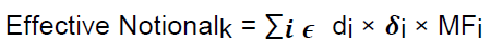
14. The Standards allows banks to choose between two options for aggregating the effective notional amounts that are calculated for each maturity category for interest rate derivatives. The primary formula is the following:

15. In this formula, D1 is the effective notional amount for maturity category 1, D2 is the effective notional amount for maturity category 2, and D3 is the effective notional amount for maturity category 3. As defined in the Standards, maturity category 1 is less than one year, maturity category 2 is one to five years, and maturity category 3 is more than five years.
16. As an alternative, the bank may choose to combine the effective notional values as the simple sum of the absolute values of D1, D2, and D3 within a hedging set, which has the effect of ignoring potential diversification benefits. That is, as an alternative to the calculation above, the bank may calculate:
|D1| + |D2| + |D3|
This alternative is a simpler calculation, but is more conservative in the sense that it always produces a larger result. To see this, note that the two calculations would give identical results only if the values 1.4 and 0.6 in the first formula are replaced with the value 2.0. Since the actual coefficient values are smaller than 2.0, the first formula gives a smaller result than the second formula. Choosing the second formula is equivalent to choosing to use the first formula with the 1.4 and 0.6 values replaced by 2.0, increasing measured CCR exposure and therefore minimum required capital.
F. Maturity Factor
17. Note that the Standards requires the use of a standard 250-day trading or business year for the calculation of the maturity factor and the MPOR. The view of the Central Bank is that a single, standardised definition of one year for this purpose will enhance comparability across banks and over time. However, the BCBS has indicated that the number of business days used for the purpose of determining the maturity factor be calculated appropriately for each transaction, taking into account the market conventions of the relevant jurisdiction. If a bank believes that use of a different definition of one year is appropriate, or would significantly reduce its compliance burden, the bank may discuss the matter with bank supervisors.
G. Delta Adjustment
18. Supervisory delta adjustments reflect the fact that the notional value of a transaction is not by itself a good indication of the associated risk. In particular, exposure to future market movements depends on the direction of the transaction and any non-linearity in the structure.
19. With respect to direction, a derivative may be long exposure to the underlying risk factor (price, rate, volatility, etc.), in which case the value of the derivative will move in the same direction as the underlying – gaining value with increases, losing value with decreases – and the delta is positive to reflect this relationship. The alternative is that a derivative may be short exposure to the underlying risk factor, in which case the value of the derivative moves opposite to the underlying – losing value with increases, and gaining value with decreases – and thus the delta is negative.
20. The non-linearity effects are prominent with transactions that involve contingent payoffs or option-like elements. Options and CDOs are notable examples. For such derivative transactions, the impact of a change in the price of the underlying instrument is not linear or one-for-one. For example, with an option on a foreign currency, when the exchange rate changes by a given amount, the change in the value of the derivative – the option contract – will almost always be less than the change in the exchange rate. Moreover, the amount by which the change is less than one-for-one will vary depending on a number of factors, including the current exchange rate relative to the exercise price of the option, the time remaining to expiration of the option, and the current volatility of the exchange rate. Without an adjustment for that difference, the notional amounts alone would be misleading indications of the potential for counterparty credit risk.
21. The supervisory delta adjustments for all derivatives are presented in the table below, which is repeated from the CCR Standards. These adjustments are defined at the trade level, and are applied to the adjusted notional amounts to reflect the direction of the transaction and its non-linearity.
22. Note that the supervisory delta adjustments for the various option transactions are closely related to the delta from the widely used Black-Scholes model of option prices, although the risk-free interest rate – which would ordinarily appear in this expression – is not included. In general, banks should use a forward price or rate, ideally reflecting any interim cash flows on the underlying instrument, as P in the supervisory delta calculation.
23. The expression for the supervisory delta adjustment for CDOs is based on attachment and detachment points for any tranche of the CDO. The precise specification (including the values of the embedded constants of 14 and 15) is the result of an empirical exercise conducted by the Basel Committee on Banking Supervision to identify a relatively simple functional form that would provide a sufficiently close fit to CDO sensitivities as reported by a set of globally active banks.
Supervisory Delta Adjustments
Type of Derivative Transaction Supervisory Delta Adjustment Purchased Call Option F Purchased Put Option F-1 Sold Call Option -F Sold Put Option 1-F Purchased CDO Tranche (Long Protection) G Sold CDO Tranche (Short Protection) -G Any Other Derivative Type, Long in the Primary Risk Factor +1 Any Other Derivative Type, Short in the Primary Risk Factor -1 Definitions
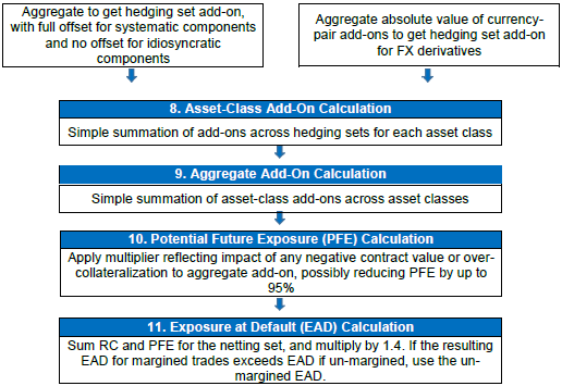
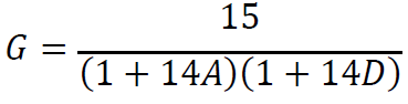
For options:
In this expression, P is the current forward value of the underlying price or rate, K is the exercise or strike price of the option, T is the time to the latest contractual exercise date of the option, σ is the appropriate supervisory volatility from Table 2, and Φ is the standard normal cumulative density function. A supervisory volatility of 50% should be used on swaptions for all currencies.
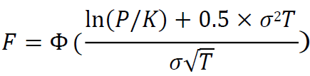
For CDO tranches:
In this expression, A is the attachment point of the CDO tranche and D is the detachment point of the CDO tranche.
H. Complex Derivatives
24. The Standards requires that complex trades with more than one risk driver (e.g. multi-asset or hybrid derivatives) must be allocated to more than one asset class when the material risk drivers span more than one asset class. The full amount of the trade must be included in the PFE calculation for each of the relevant asset classes. Asset-class allocation of complex derivatives is a point of national discretion in the Basel framework, and the Central Bank believes that requiring banks to identify such trades and allocate them accordingly places appropriate responsibility on banks that choose to engage in such trades.
25. Examples of derivatives that reference the basis between two risk factors and are denominated in a single currency (basis transactions) include three-month Libor versus six-month Libor, three-month Libor versus three-month T-Bill, one-month Libor versus OIS rate, or Brent Crude oil versus Henry Hub gas. These examples are provided as illustrations, and do not represent an exhaustive list.
26. Hedging sets for derivatives that reference the volatility of a risk factor (volatility transactions) must follow the same hedging set construction outlined in the Standards for derivatives in that asset class; for example, all equity volatility transactions form a single hedging set. Examples of volatility transactions include variance and volatility swaps, or options on realized or implied volatility.
I. Unrated Reference Assets
27. The supervisory factor for credit derivatives depends on the credit rating of the underlying reference asset. The Basel framework does not provide a specific treatment of unrated reference assets. The Central Bank believes that credit derivatives on unrated reference entities are likely to be rare. However, for the sake of completeness, the Standards requires that any such credit derivatives be treated in a manner that is broadly consistent with the treatment of unrated entities in other aspects of the risk-based capital framework, through use of a Supervisory Factor corresponding to BBB or BB ratings as described in the Standards.
28. For an entity for which a credit rating is not available, a bank should use the Supervisory Factor corresponding to BBB. However, where the exposure is associated with an elevated risk of default, the bank should use the Supervisory Factor for BB. In this context, “elevated risk of default” should also be understood to include instances in which it is difficult or impossible to assess adequately whether the exposure has high risk of loss due to default by the obligor. A bank trading credit derivatives referencing unrated entities should conduct their own analysis to examine this risk.
J. Commodity Derivatives
29. Note that the Standards defines the term “commodity type” for purposes of calculation of exposure for CCR. A commodity type is defined as a set of commodities with broadly similar risk drivers, such that the prices or volatilities of commodities of the same commodity type may reasonably be expected to move with similar direction and timing and to bear predictable relationships to one another. For example, a commodity type such as coal might include several types of coal, and a commodity type such as oil might include oil of different grades from different sources. The prices of commodities of a given type may not move precisely in lock step, but they are likely to move in the same direction at roughly the same time, due to their dependence on common forces in commodity markets. Long and short trades within a single commodity type can be fully offset.
30. For commodity derivatives, defining individual commodity types is operationally difficult. In fact, it is generally not possible to fully specify all relevant distinctions between commodity types, and as a result, a single commodity type is likely to include individual commodities that in practice differ to some extent in the dynamic behaviour they exhibit. As a result, not all basis risk is likely to be captured. Nonetheless, banks should attempt to minimize unrecognized basis risk through sound definitions of commodity types.
31. The Standards requires a bank to establish appropriate governance processes for the creation and maintenance of the list of defined commodity types used by the bank for CCR calculations, with clear definitions and independent internal review or validation processes to ensure that commodities grouped as a single type are in fact similar. A bank can only use the specifically defined commodity types it has established through its adequately controlled internal processes.
32. Trades within the same commodity hedging set (Energy, Metals, Agriculture, and Other) enjoy partial offsetting through the use of correlation values established in the Standards, with correlation values varying by asset subclass. More specifically, partial offsetting applies only to the systematic component, not the issuer-specific or idiosyncratic component. Note that Electricity is a sub-class of the Commodity asset class, but is itself part of the broader Energy hedging set, rather than constituting a distinct hedging set.
K. Single-Name and Index Derivatives
33. For credit derivatives, there is one credit reference entity for each reference debt instrument that underlies a single-name transaction allocated to the credit risk category. Single-name transactions should be assigned to the same credit reference entity only where the underlying reference debt instrument of those transactions is issued by the same issuer.
34. The approach for establishing the reference entity for equity derivatives should correspond to the general approach for credit derivatives.
35. For credit derivatives with indices as the underlying instrument, there should be one reference entity for each group of reference debt instruments or single-name credit derivatives that underlie a multi-name transaction. Multi-name transactions should be assigned to the same credit reference entity only where the group of underlying reference debt instruments or single-name credit derivatives of those transactions has the same constituents. The determination of whether an index is investment grade or speculative grade should be based on the credit quality of the majority of its individual constituents.
36. Again, the approach for equity index derivatives should follow the general approach for credit index derivatives.
L. Special Cases of Margin Agreements
37. When multiple margin agreements apply to a single netting set, the netting set should be broken down into sub-netting sets that align with the respective margin agreement for calculating both RC and PFE.
38. When a single margin agreement applies to multiple netting sets, RC at any given time is determined by the sum of two terms. The first term is equal to the un-margined current exposure of the bank to the counterparty aggregated across all netting sets within the margin agreement reduced by the positive current net collateral (i.e. collateral is subtracted only when the bank is a net receiver of collateral). The second term is non-zero only when the bank is a net poster of collateral: it is equal to the current net posted collateral (if there is any) reduced by the un-margined current exposure of the counterparty to the bank aggregated across all netting sets within the margin agreement. Net collateral available to the bank should include both VM and NICA. Mathematically, RC for the entire margin agreement is:
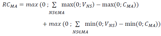
where the summation NS ∈ MA is across the netting sets covered by the margin agreement (hence the notation), VNS is the current mark-to-market value of the netting set NS and CMA is the cash equivalent value of all currently available collateral under the margin agreement.
39. An alternative description of this calculation is as follows:
Step 1: Compute the net value, positive or negative, of each netting set. These calculated values correspond to the terms VNS in the expression above.
Step 2: Sum the values of all netting sets with positive value, to get Total Positive Value (TPV). This corresponds to the term in the expression above: 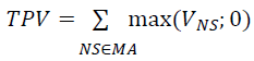
Step 3: Sum the values of all of netting sets with negative value, to get Total Negative Value (TNV). This corresponds to the term in the expression above: 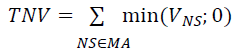
Step 4: Calculate the net current cash value of collateral, including NICA and VM. This corresponds to the term CMA in the expression above. If the bank is net holder of collateral, then CMA is positive; it is the net value held (NVH). If the bank is a net provider of collateral, then CMA is negative, and its absolute value is the net value provided (NVP). Note that either NVH>0 and NVP=0, or NVP>0 and NVH=0.
One of the following cases then applies:
Step 5a: If NVH>0 (so NVP=0), then RC = TPV – NVH, but with a minimum of zero – that is, RC cannot be negative.
or
Step 5b: If NVH=0 (so NVP>0), then RC = TPV + NVP – TNV, but with a minimum of TPV – that is, RC cannot be less than TPV.
40. To calculate PFE when a single margin agreement applies to multiple netting sets, netting set level un-margined PFEs should be calculated and aggregated, i.e. PFE should be calculated as the sum of all the individual netting sets considered as if they were not subject to any form of margin agreement.

III. Summary of the EAD Calculation Process
IV. Frequently Asked Questions
A. Netting
Question A1: Does a bank need written approval for each netting agreement it has in place, or will the Central Bank provide a list of pre-approved jurisdictions or counterparties?
The bank should establish an internal process that considers the factors identified in the Standards. That process should be subject to internal review and challenge per the Standards. The Central Bank will review the identification of netting sets as part of the supervisory process, and notify the bank of any determinations that netting is not appropriate. The Central Bank will not provide a list of pre-approved jurisdictions or counterparties.Question A2: Do amendments to existing netting agreements require approval from the Central Bank?
Amendments that do not raise new questions about the validity of netting need not be raised to the Central Bank for consideration.Question A3: What if netting is not valid? Can netting sets still be used for the calculation?
If the requirements of the Standards for recognition of netting are not satisfied, then each transaction is its own netting set – a netting set consisting of a single transaction – and many of the calculations are much simpler.Question A4: Is use of the standard ISDA agreement sufficient to apply netting?
No, use of the standard ISDA agreement is not in itself sufficient to demonstrate that netting is valid and legally enforceable in the relevant jurisdictions under the requirements of the Standards.Question A5: Can we treat trades with a UAE counterparty (UAE Bank or Foreign Bank operating in the UAE) having a signed ISDA / CSA as a netting set even though the UAE is not a netting jurisdiction?
No, as noted above, use of the standard ISDA agreement is not in itself sufficient to demonstrate that netting is valid and legally enforceable in the relevant jurisdictions under the requirements of the Standards, and is not a replacement for a determination regarding the legal enforceability of netting.Question A6: If there is no netting agreement of any sort in place, what would the treatment be for trades with negative mark to market? Will they be included or excluded from the exposure calculation?
Trades with negative value have RC=0, but still have counterparty credit risk, which will be reflected in the calculation of the PFE component of exposure.B. Collateral
Question B1: What haircuts should be applied to collateral for the calculations of exposure net of collateral?
Banks should apply the standard supervisory haircuts from the capital framework.Question B2: If a counterparty places initial cash margin against a derivatives facility, but has no signed ISDA / CSA in place, can this cash margin be considered as collateral for Replacement Cost calculations?
Yes, provided the arrangement allows the bank to retain the cash in the event of a default by the counterparty.Question B3: Can collateral received under a CSA be considered as part of the RC calculation in absence of a netting agreement?
Yes. Note that in the absence of netting, the netting set would consist of a single trade and any collateral corresponding to that trade.C. Classification of Trades
Question C1: For a currency swap involving principal and interest exchange, since there is exchange rate risk in addition to interest rate risk, do we need to assign the notional to both the currency and interest rate classes?
Yes, derivatives with exposure to more than one primary risk factor should be allocated to all relevant asset classes for the PFE calculation, so this transaction should be included in its full amount in both the Foreign Exchange hedging set and the Interest Rate hedging set.Question C2: In a cross-currency swap with principal exchange at the beginning and at the end, and with fixed-rate to fixed-rate interest exchange so that there is no interest rate risk, should this trade be included only in the foreign currency category?
Yes, it should be treated as FX exposure.Question C3: Is there any prescribed PFE treatment for a derivative such as a weather derivative?
Derivatives with "unusual" underlying such as weather or mortality are included in the "Other" hedging set within the Commodity asset class.Question C4: Can trades with gold as the underlying asset be treated as currency derivatives?
No. Although gold often has been grouped with foreign exchange historically, for the CCR Standards it is to be treated as a metal within the commodity asset class.D. Supervisory Delta Adjustment
Question D1: What is the Supervisory Delta for FX Swaps and FX Forwards?
These are linear contracts, so the Supervisory Delta is either +1 (for long positions) or -1 (for short positions).Question D2: The Standards states that the Supervisory Delta for a short position (one that is not an option or CDO) should be -1. However, if netting is not permitted, should the Supervisory Delta be set to +1 for all the short (as well as the long) positions?
In principle, the Supervisory Delta should be -1 if the position is short. However, in the case of a single-trade netting set, there is no possibility of offsetting, so the sign of the Supervisory Delta does not affect the calculation.Question D3: In the case of an option strategy such as a straddle or strangle involving more than one type of option (e.g. a long call and a long put), which Supervisory Delta should be used?
In the case of positions that involve combinations of options, the position should be decomposed into its simpler option components, appropriate Supervisory Deltas determined for each component, and the weighted average Supervisory Delta applied to the position as a whole.Question D4: In the case of an option strategy involving multiple options with only one leg having a possibility of exercise, can we consider this structure as a "short" position if we are net receiver of the premium and a "long" position if we are net payer of premium?
As noted above, in the case of positions that involve combinations of options, the position should be decomposed into its simpler option components, appropriate Supervisory Deltas determined for each component, and the weighted average Supervisory Delta applied to the position as a whole. In this case, some of the Supervisory Deltas would be positive, and some would be negative. The sign of the overall Supervisory Delta would depend on the relative size of the positions, and the associated magnitude (in absolute value) of the deltas.Question D5: Should the same set of Supervisory Deltas be used in the case of path dependent options such as barrier options, or other complex options? For such products, the simple option delta formula may not be appropriate.
Banks should apply the standardised formulas for the CCR calculations, including the Supervisory Delta adjustment for all options. Note that use of a single, simplified formula for the Supervisory Delta for options is a feature of the Standardised Approach. Like all standardised approaches, the SA-CCR involves numerous trade-offs between precision and simplicity. Many other aspects of the Standardised Approach use approximations, such as the assumption that a single correlation should be used for all commodity derivatives, or the use of a single volatility for all FX options. Banks should certainly use more analytically appropriate deltas for internal purposes such as valuation and risk management.E. Hedging Sets
Question E1: Can different floating rates within the same base currency be included in single hedging set?
Yes, for interest rate derivatives, all rates within one base currency should be included in a single hedging set.Question E2: Is it possible to determine a hedging set in the absence of a netting set?
Yes, without a netting set, the hedging set would consist of a single transaction, and the add-on would be simply the effective notional amount of that one transaction.F. Maturity and Supervisory Duration
Question F1: For Supervisory Duration, should S and E be based on original maturity or residual maturity?
Calculation of S and E should be computed relative to the current date, not the date at which the trade was initiated; hence, they are most similar to residual maturity.Question F2: When calculating the remaining maturity in business days, should we follow the business calendar given in the master agreement, or the business calendar within the jurisdiction in which the bank is operating?
The Basel Committee has provided guidance that the number of business days used for the purpose of determining the maturity factor must be calculated appropriately for each transaction, taking into account the market conventions of the relevant jurisdiction. The Central Bank follows this approach as well.Question F3: What is the maturity factor if the remaining maturity is greater than 250 business days?
In that case, the maturity factor for the CCR calculations is equal to 1.0.Question F4: What would be the maturity of a derivative with multiple exchanges of notional over a period of time?
The maturity date is the date of the final exchange or payment under the contract.Question F5: What is the Maturity Factor for deals such as callable range accruals where the call date is less than 1 year, but the deal maturity is more than 1 year?
Since the deal maturity is more than one year, the Maturity Factor would be equal to 1.0.G. Other
Question G1: For certain capital calculations in the past, exchange rate contracts with an original maturity of 14 calendar days or less were excluded from certain capital requirements. Is that applicable for the CCR Standards?
No, all in-scope exchange rate contracts must be included, regardless of original or remaining maturity.Question G2: A single hedging set might include derivatives on underlying rates, prices, or entities that span different Basel categories (e.g. corporates, financials, sovereigns); do these need to be calculated separately in order to compute and report RWA in the format required by the reporting template?
No, the risk-weight, and the category for reporting in the Central Bank’s template, depends on the nature of the counterparty, not the nature of the underlying reference asset. The counterparty for any netting set will fall into one and only one category for risk weighting and for reporting.Question G3: For a variable notional swap, how should the average notional be calculated?
Use the time-weighted average notional in the CCR calculations.Question G4: Should the current spot rate be used to compute adjusted notional?
Yes, the current spot rate should be used.Question G5: Bank ask in case of calculating discounted counterparty exposure is a double count and will inflate CVA Capital charge given SA-CCR EAD already factors in maturity adjustment while computing adjusted notional which is product of trade notional & supervisory duration?
The use of the discount factor in the CVA capital charge does not result in double counting. While there is superficial similarity between the supervisory duration (SD) adjustment in SA-CCR and the discount factor (DF) in CVA, they are actually capturing different aspects of risk exposure. The use of SD in SA-CCR adjusts the notional amount of the derivatives to reflect its sensitivity to changes in interest rates, since longer-term derivatives are more sensitive to rate changes than are shorter-term derivatives. In contrast, the use of DF in the CVA calculation reflects the fact that a bank is exposed to CVA risk not only during the first year of a derivative contract, but over the life of the contract; the DF term recognizes the present value of the exposure over the life of the contract. Thus, these two factors, although they have similar functional forms and therefore appear somewhat similar, are not in fact duplicative.V. Illustrations of EAD Calculations
A. Illustration 1
Consider a netting set with three interest rates derivatives: two fixed versus floating interest rate swaps and one purchased physically settled European swaption. The table below summarizes the relevant contractual terms of the three derivatives. All notional amounts and market values in the table are given in USD. We also know that this netting set is not subject to a margin agreement and there is no exchange of collateral (independent amount/initial margin) at inception.
Trade # Nature Residual maturity Base currency Notional (thousands) Pay Leg (*) Receive Leg (*) Market value (thousands) 1 Interest rate swap 10 years USD 10,000 Fixed Floating 30 2 Interest rate swap 4 years USD 10,000 Floating Fixed -20 3 European swaption 1 into 10 years EUR 5,000 Floating Fixed 50 (*) For the swaption, the legs are those of the underlying swap.
The EAD for un-margined netting sets is given by:
EAD = 1.4 * (RC + PFE)
1. Replacement Cost Calculation
The replacement cost is calculated at the netting set level as a simple algebraic sum (floored at zero) of the derivatives’ market values at the reference date. Thus, using the market values indicated in the table (expressed in thousands):
RC = max {V - C; 0} = max {30 - 20 + 50; 0} = 60
Since V-C is positive (equal to V of 60,000), the value of the multiplier is 1, as explained in the Standards.
2. Potential Future Exposure Calculation
All the transactions in the netting set belong to the interest rate asset class. So the Add-on for interest rate class must be calculated as well as the multiplier since
PFE = multiplier × Add-onagg
For the calculation of the interest rate add-on, the three trades must be assigned to a hedging set (based on the currency) and to a maturity category (based on the end date of the transaction). In this example, the netting set is comprised of two hedging sets, since the trades refer to interest rates denominated in two different currencies (USD and EUR). Within hedging set “USD”, Trade 1 falls into the third maturity category (>5 years) and Trade 2 falls into the second maturity category (1-5 years). Trade 3 falls into the third maturity category (>5 years) of hedging set “EUR”.
S and E represent the start date and end date, respectively, of the time period referenced by the interest rate transactions.
Trade # Hedging set Time bucket Notional (thousands) S E 1 USD 3 10,000 0 10 2 USD 2 10,000 0 4 3 EUR 3 5,000 1 11 The following table illustrates the steps typically followed for the add-on calculation:
Steps Activities 1. Calculate Effective Notional Calculate supervisory duration
Calculate trade-level adjusted notional as trade notional (in domestic currency) × supervisory duration
Effective notional for each maturity category = Σ(trade-level adjusted notional × supervisory delta × maturity factor), with full offsetting for each of the three maturity categories, in each hedging set (that is, same currency)2. Apply Supervisory Factors Add-on for each maturity category in a hedging set (that is, same currency) = Effective Notional Amount for maturity category × interest rate supervisory factor 3. Apply Supervisory Correlations Add-on for each hedging set = Σ(Add-ons for maturity categories), aggregating across maturity categories for a hedging set. One hedging set for each currency. 4. Aggregate Simple summation of the add-ons for the different hedging sets Calculate Effective Notional Amount
The adjusted notional of each trade is calculated by multiplying the notional amount by the calculated supervisory duration SD as defined in the Standards.
d = Trade Notional × SD = Trade Notional × (exp(-0.05×S) – exp(-0.05 × E)) / 0.05
Trade Notional Amount Time Bucket S E Supervisory Duration SD Adjusted Notional d Trade 1 10,000,000 3 0 10 7.869386806 78,693,868.06 Trade 2 10,000,000 2 0 4 3.625384938 36,253,849.38 Trade 3 5,000,000 3 1 11 7.485592282 37,427,961.41 Calculate Maturity Category Effective Notional
A supervisory delta is assigned to each trade in accordance with the Standards. In particular:
- •Trade 1 is long in the primary risk factor (the reference floating rate) and is not an option so the supervisory delta is equal to 1.
- •Trade 2 is short in the primary risk factor and is not an option; thus, the supervisory delta is equal to -1.
- •Trade 3 is an option to enter into an interest rate swap that is short in the primary risk factor and therefore is treated as a purchased put option. As such, the supervisory delta is determined by applying the relevant formula using 50% as the supervisory option volatility and 1 (year) as the option exercise date. Assume that the underlying price (the appropriate forward swap rate) is 6% and the strike price (the swaption’s fixed rate) is 5%.
The trade-level supervisory delta is therefore:
Trade Delta Instrument Type Trade 1 1 linear, long (forward and swap) Trade 2 -1 linear, short (forward and swap) Trade 3 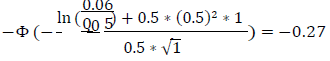
purchased put option The Maturity Factor MF is 1 for all the trades since they are un-margined and have remaining maturities in excess of one year.
Based on the maturity categories, the Effective Notional D for the USE and EUR hedging sets at the level of the maturity categories are as shown in the table below:
Hedging Set Time Bucket Adjusted Notional Supervisory Delta Maturity Factor Maturity category-level Effective Notional D HS 1 (USD) 3 78,693,868 1 1 78,693,868 2 36,253,849 -1 1 -36,253,849 HS 2 (EUR) 3 37,427,961 -0.27 1 -10,105,550 In particular:
Hedging set USD, time bucket 3: D = 1 * 78,693,868 * 1 = 78,693,868
Hedging set USD, time bucket 2: D = -1 * 36,253,849 * 1 = -36,253,849
Hedging set EUR, time bucket 3: D = -0.27 * 37,427,961 * 1 = -10,105,550
Apply Supervisory Factor
The add-on must be calculated for each hedging set.
For the USD hedging set there is partial offset between the two USD trades:
Effective notional(IR) USD = [D22 + D32 + 1.4 x D2 x D3]1/2
= [(-36,253,849)2 + 78,693,8682 + 1.4 × (-36,253,849) × 78,693,868]1/2
= 59,269,963
For the Hedging set EUR there is only one trade (and one maturity category):
Effective notional(IR)EUR = 10,105,550
In summary:
Hedging set Time Bucket Maturity category-level Effective Notional Dj,k Hedging Set level Effective Notional Dj,k (IR) HS 1 (USD) 3 78,693,868 59,269,963
(Partial offset)2 -36,253,849 HS 2 (EUR) 3 -10,105,550 10,105,549.58 Aggregation of the calculated add-ons across different hedging sets:
Effective Notional(IR) = 59,269,963 + 10,105,550 = 69,375,513 (No offset between hedging sets) The asset class is interest rates; thus the applicable Supervisory factor is 0.50%. As a result:
Add-on = SF × Effective Notional = 0.005 × 69,375,513 = 346,878
Supervisory Correlation Parameters
Correlation is not applicable to the interest rate asset class, and there is no other asset class in the netting set in this example.
Add-on Aggregation
For this netting set, the interest rate add-on is also the aggregate add-on because there are no trades assigned to other asset classes. Thus, the aggregate add-on = 346,878
Multiplier
The multiplier is given by:
multiplier = min { 1; Floor+(1-Floor) × exp [(V-C) /(2 ×(1-Floor)×Add-onagg)]}
= min {1; 0.05 + 0.95 × exp [60,000 / (2 × 0.95 × 346,878]}
=1
Final Calculation of PFE
In this case the multiplier is equal to one, so the PFE is the same as the aggregate Add-On:
PFE = multiplier × Add-onagg = 1 × 346,878 = 346,878
3. EAD Calculation
The exposure EAD to be risk weighted for counterparty credit risk capital requirements purposes is therefore
EAD = 1.4 * (RC + PFE) = 1.4 x (60,000 + 346,878) = 569,629
B. Illustration 2
Consider a netting set with three credit derivatives: one long single-name CDS written on Firm A (rated AA), one short single-name CDS written on Firm B (rated BBB), and one long CDS index (investment grade). All notional amounts and market values are denominated in USD. This netting set is not subject to a margin agreement and there is no exchange of collateral (independent amount/initial margin) at inception. The table below summarizes the relevant contractual terms of the three derivatives.
Trade # Nature Reference entity / index name Rating reference entity Residual maturity Base currency Notional (thousands) Position Market value (thousands) 1 Single-name CDS Firm A AA 3 years USD 10,000 Protection buyer 20 2 Single-name CDS Firm B BBB 6 years EUR 10,000 Protection seller -40 3 CDS index CD X.IG Investment grade 5 years USD 10,000 Protection buyer 0 According to the Standards, the EAD for un-margined netting sets is given by:
EAD = 1.4 * (RC + PFE)
1. Replacement Cost Calculation
The replacement cost is calculated at the netting set level as a simple algebraic sum (floored at zero) of the derivatives’ market values at the reference date. Thus, using the market values indicated in the table (expressed in thousands):
RC = max {V - C; 0} = max {20 - 40 + 0; 0} = 0
Since V-C is negative (i.e. -20,000), the multiplier will be activated (i.e. it will be less than 1). Before calculating its value, the aggregate add-on needs to be determined.
2. Potential Future Exposure Calculation
The following table illustrates the steps typically followed for the add-on calculation:
Steps Activities 1. Calculate Effective Notional Calculate supervisory duration
Calculate trade-level adjusted notional = trade notional (in domestic currency) × supervisory duration
Calculate trade-level effective notional amount = trade-level adjusted notional × supervisory delta × maturity factor
Calculate effective notional amount for each entity by summing the trade-level effective notional amounts for all trades referencing the same entity (either a single entity or an index) with full offsetting2. Apply Supervisory Factors Add-on for each entity in a hedging set = Entity-level Effective Notional Amount × Supervisory Factor, which depends on entity’s credit rating (or investment/speculative for index entities) 3. Apply Supervisory Correlations Entity-level add-ons are divided into systematic and idiosyncratic components weighted by the correlation factor 4. Aggregate Aggregation of entity-level add-ons with full offsetting in the systematic component and no offsetting in the idiosyncratic component Effective Notional Amount
The adjusted notional of each trade is calculated by multiplying the notional amount with the calculated supervisory duration SD specified in the Standards.
d= Trade Notional × SD = Trade Notional × {exp(-0.05×S) – exp(-0.05 × E)} / 0.05
Trade Notional Amount S E Supervisory Duration SD Adjusted Notional d Trade 1 10,000,000 0 3 2.785840471 27,858,405 Trade 2 10,000,000 0 6 5.183635586 51,836,356 Trade 3 10,000,000 0 5 4.423984339 44,239,843 The appropriate supervisory delta must be assigned to each trade: in particular, since Trade 1 and Trade 3 are long in the primary risk factor (CDS spread), their delta is 1; in contrast, the supervisory delta for Trade 2 is -1.
Trade Delta Instrument Type Trade 1 1 linear, long (forward and swap) Trade 2 -1 linear, short (forward and swap) Trade 3 1 linear, long (forward and swap) Thus, the entity-level effective notional is equal to the adjusted notional times the supervisory delta times the maturity factor (where the maturity factor is 1 for all three derivatives).
Trade Adjusted Notional Supervisory Delta Maturity Factor Entity Level Effective Notional Trade 1 27,858,405 1 1 27,858,405 Trade 2 51,836,356 -1 1 -51,836,356 Trade 3 44,239,843 1 1 44,239,843 Supervisory Factor
The add-on must now be calculated for each entity. Note that all derivatives refer to different entities (single names/indices). A supervisory factor is assigned to each single-name entity based on the rating of the reference entity, as specified in Table 1 in the relevant Standards. This means assigning a supervisory factor of 0.38% for AA-rated firms (Trade 1) and 0.54% for BBB-rated firms (for Trade 2). For CDS indices (Trade 3), the supervisory factor is assigned according to whether the index is investment or speculative grade; in this example, its value is 0.38% since the index is investment grade.
Asset Class Subclass ρ SF Credit, Single Name AA 50% 0.38% Credit, Single Name BBB 50% 0.54% Credit, Index IG 80% 0.38% Thus, the entity level add-ons are as follows:
Add-on(Entity) = SF × Effective Notional
Trade Effective Notional Supervisory factor SF Add-on (Entity) Trade 1 27,858,405 0.38% 105,862 Trade 2 -51,836,356 0.54% -279,916 Trade 3 44,239,843 0.38% 168,111 Supervisory Correlation Parameters
The add-on calculation separates the entity level add-ons into systematic and idiosyncratic components, which are combined through weighting by the correlation factor. The correlation parameter ρ is equal to 0.5 for the single-name entities (Trade 1-Firm A and Trade 2-Firm B) and 0.8 for the index (Trade 3-CDX.IG) in accordance with the requirements of the Standards.
Add-on(Credit) = [ [ ∑k ρk CR × Add-on (Entityk) ]2 + ∑k (1- (ρk CR)2) × (Add-on (Entityk))2]1/2
Trade ρ Add-on(Entityk) ρ × Add-on(Entityk) (1 – ρ2) (1 – ρ2) × (Add-on(Entityk))2 Trade 1 50% 105,862 52,931 0.75 8,405,062,425 Trade 2 50% -279,916 -139,958 0.75 58,764,860,350 Trade 3 80 % 168,111 134,489 0.36 10,174,120,000 Systematic Component 47,462 Idiosyncratic Component 77,344,042,776 Full offsetting No offsetting Add-on Aggregation
For this netting set, the interest rate add-on is also the aggregate add-on because there are no trades assigned to other asset classes. Thus, the aggregate add-on = 346,878
Aggregation of entity-level add-ons with full offsetting in the systematic component and no offsetting benefit in the idiosyncratic component.
Systematic Component 47,462 Idiosyncratic Component 77,344,042,776 Thus,
Add-on = [ (47,462)2 + 77,344,042,776 ]1/2 = 282,129
Multiplier
The multiplier is given by
multiplier = min {1; Floor+(1-Floor) × exp [(V-C)/(2×(1-Floor)×Add-onagg)]}
= min {1; 0.05 + 0.95 × exp [-20,000 / (2 × 0.95 × 282,129)]}
=0.96521
Final Calculation of PFE
PFE = multiplier × Add-onagg = 0.96521 × 282,129= 272,313
3. EAD Calculation
The exposure that would be risk-weighted for the purpose of counterparty credit risk capital requirements is therefore:
EAD = 1.4 * (RC + PFE) = 1.4 x (0 + 272,313) = 381,238
C. Illustration 3
Consider a netting set with three commodity forward contracts. All notional amounts and market values are denominated in USD. This netting set is not subject to a margin agreement and there is no exchange of collateral (independent amount/initial margin) at inception. The table below summarizes the relevant contractual terms of the three commodity derivatives.
Trade # Nature Underlying Position Direction Residual maturity Notional (thousands) Market value (thousands) 1 Forward (WTI)
Crude OilProtection Buyer Long 9 months 10,000 -50 2 Forward (Brent)
Crude OilProtection Seller Short 2 years 20,000 -30 3 Forward Silver Protection Buyer Long 5 years 10,000 100 1. Replacement Cost Calculation
The replacement cost is calculated at the netting set level as a simple algebraic sum (floored at zero) of the derivatives’ market values at the reference date, provided that value is positive. Thus, using the market values indicated in the table (expressed in thousands):
RC = max {V - C; 0} = max {100 - 30 - 50; 0} = 20
The replacement cost is positive and there is no exchange of collateral (so the bank has not received excess collateral), which means the multiplier will be equal to 1.
2. Potential Future Exposure Calculation
The following table illustrates the steps typically followed for the add-on calculation, for each of the four commodity hedging sets with non-zero exposure:
Steps Activities 1. Calculate Effective Notional Calculate trade-level adjusted notional = current price × number of units referenced by derivative
Calculate trade-level effective notional amount = trade-level adjusted notional × supervisory delta × maturity factor
Calculate effective notional for each commodity-type = Σ(trade-level effective notional) for trades referencing the same commodity type, with full offsetting in commodity type2. Apply Supervisory Factors Add-on for each commodity type in a hedging set = Commodity-type Effective Notional Amount × Supervisory Factor 3. Apply Supervisory Correlations Commodity-type add-ons are divided into systematic and idiosyncratic components weighted by the correlation factor 4. Aggregate Aggregation of commodity-type add-ons with full offsetting in the systematic component and no offsetting in the idiosyncratic component
Simple summation of absolute values of add-ons across the four hedging setsEffective Notional Amount
Trade-level Adjusted Notional calculation for each commodity derivative trade:
di(COM) = current price per unit × number of units in the trade
Trade Current price per unit (unit is barrel for oil; ounces for silver) Number of units in the trade Adjusted Notional Trade 1 100 100 barrels 10,000 Trade 2 100 200 barrels 20,000 Trade 3 20 500 ounces 10,000 The appropriate supervisory delta must be assigned to each trade:
Trade Delta Instrument Type Trade 1 1 linear, long (forward & swap) Trade 2 -1 linear, short (forward & swap) Trade 3 1 linear, long (forward & swap) Since the remaining maturity of Trade 1 is less than a year, at nine months (approximately 187 business days), and the trade is un-margined, its maturity factor is scaled down by the square root of 187/250 in accordance with the requirements of the Standards. On the other hand, the maturity factor is 1 for Trade 2 and for Trade 3, since the remaining maturity of those two trades is greater than one year and they are un-margined.
The trade-level effective notional is equal to the adjusted notional times the supervisory delta times the maturity factor. The basic difference between the WTI and Brent forward contracts effectively is ignored since they belong to the same commodity type, namely “Crude Oil” within the “Energy” hedging set, thus allowing for full offsetting. (In contrast, if one of the two forward contracts were on a different commodity type within the “Energy” hedging set, such as natural gas, with the other on crude oil, then only partial offsetting would have been allowed between the two trades.) Therefore, Trade 1 and Trade 2 can be aggregated into a single effective notional, taking into account each trade’s supervisory delta and maturity factor.

Hedging Set Commodity Type Trade Adjusted Notional Supervisory Delta Maturity Factor Effective Notional Energy Crude Oil Trade 1 10,000 1 10,000 x 1 x 0.865 + 20,000x(-1)x1 =-11,350 (full off-setting within the ‘Crude Oil’ commodity type) Energy Crude Oil Trade 2 20,000 -1 1 Metals Silver Trade 3 10,000 1 1 10,000 Supervisory Factor
For each commodity-type in a hedging set, the effective notional amount must be multiplied by the correct Supervisory Factor (SF). As described in the Standards, the Supervisory Factor for both the Crude Oil commodity type in the Energy hedging set and the Silver commodity type in the Metals hedging set is SF=18%.
Thus, the add-on by hedging set and commodity type is as follows:
Add-on(Typekj) = SFTypek(Com) × Effective NotionalTypek(Com)
Hedging Set Commodity Type Effective Notional Supervisory Factor SF Add-on by HS and Commodity type Energy Crude Oil -11,350 18% -2,043 Metals Silver 10,000 18% 1,800 Supervisory Correlation Parameters
The commodity-type add-ons in a hedging set are decomposed into systematic and idiosyncratic components. The commodity subclass correlations parameters are as stated in the Standards, in this case 40% for commodities.
Thus, the hedging set level add-ons are calculated for each commodity hedging set:
Add-on(COM) = [( Σk ρj(COM) × Add-on (Typekj) )2 + Σk (1- (ρj(COM) )2) × (Add-on (Type j))2]k1/2
Hedging Set Commodity Type ρ Add-on(Typek) Systematic Component (ρ × Add-on(Typek))2 (1 – ρ2) Idiosyncratic Component (1 – ρ2) x (Add-on(Typek)) 2 Add-onj (Only one commodity type in each HS) Energy Crude Oil 40% -2,043 (-817)2 0.84 0.84 × (-2,043)2 2,043 Metals Silver 40% 1,800 (720)2 0.84 0.84 × (1,800)2 1,800 However, in this example, since only one commodity type within the “Energy” hedging set is populated (i.e. all other commodity types within that hedging set have a zero add-on), the resulting add-on for the hedging set is the same as the add-on for the commodity type. This calculation shows that when there is only one commodity type within a commodity hedging set, the hedging-set add-on is equal to the absolute value of the commodity-type add-on. (The same comment applies to the commodity type “Silver” in the “Metals” hedging set.)
Add-on Aggregation
Aggregation of commodity-type add-ons uses full offsetting in the systematic component and no offsetting benefit in the idiosyncratic component in each hedging set. As noted earlier, in this example there is only one commodity type per hedging set, which means no offsetting benefits. Computing the simple summation of absolute values of add-ons for the hedging sets:
Add-on = Σj Add-onj
Add-On = 2,043 + 1,800 = 3,843
Multiplier
The multiplier is given by
multiplier = min {1; Floor+(1-Floor) × exp [(V-C)/(2×(1-Floor)×Add-onagg)]}
= min {1; 0.05 + 0.95 × exp [20 / (2 × 0.95 × 3,843)]}
= 1, since V-C is positive.
Final Calculation of PFE
PFE = multiplier × Add-onagg = 1 × 3,843 = 3,843
3. EAD Calculation
The exposure EAD to be risk weighted for counterparty credit risk capital requirements purposes is therefore
EAD = 1.4 * (RC + PFE) = 1.4 x (20 + 3,843) = 5,408
VI. Illustrations of Replacement Cost Calculations with Margining
Calculation of Replacement Cost (RC) depends whether or not a trade is collateralized, as illustrated below and in the summary table.
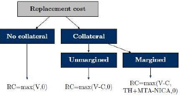

Transaction Characteristics Replacement Cost (RC) No collateral Value of the derivative transactions in the netting set, if that value is positive (else RC=0) Collateralized, no margin Value of the derivative transactions in the netting set minus the value of the collateral after applicable haircuts, if positive (else RC=0) Collateralized and margined Same as the no margin case, unless TH+MTA-NICA (see definitions below) is greater than the resulting RC - •TH = positive threshold before the counterparty must send collateral to the bank
- •MTA = minimum transfer amount applicable to the counterparty
- •NICA = net independent collateral amount other than variation margin (unsegregated or segregated) posted to the bank, minus the unsegregated collateral posted by the bank. The quantity TH + MTA – NICA represents the largest net exposure, including all collateral held or posted under the margin agreement that would not trigger a collateral call.
A. Illustration 1: Margined Transaction
A bank has AED80 million in trades with a counterparty. The bank currently has met all past variation margin (VM) calls, so the value of trades with the counterparty is offset by cumulative VM in the form of cash collateral received. Furthermore, an “Independent Amount” (IA) of AED 10 million was agreed in favour of the bank, and none in favour of its counterparty. This leads to a credit support amount of AED 90 million (80 million plus 10 million), which is assumed to have been fully received as of the reporting date. There is a small “Minimum Transfer Amount” (MTA) of AED1 million, and a “Threshold” (TH) of zero.
In this example, the V-C term in the replacement cost (RC) formula is zero, since the value of the trades is more than offset by collateral received; AED80 million – AED90 million = -10 million. The term (TH + MTA - NICA) is -9 million (0 TH + 1 million MTA - 10 million of NICA held). Using the replacing cost formula:
RC = MAX {(V-C), (TH+MTA-NICA), 0}
= MAX{(80-90),(0+1-10),0}
= MAX{-10,-9,0} = 0
Because both V-C and TH+MTA-NICA are negative, the replacement cost is zero. This occurs because of the large amount of collateral posted by the bank’s counterparty.
B. Illustration 2: Initial Margin
A bank, in its capacity as clearing member of a CCP, has posted VM to the CCP in an amount equal to the value of the trades it has with the CCP. The bank has posted AED10 million in cash as initial margin, and the initial margin is held in such a manner as to be bankruptcy-remote from the CCP. Assume that the value of trades with the CCP are -50 million, and the bank has posted AED50 million in VM to the CCP. Also assume that MTA and TH are both zero under the terms of clearing at the CCP.
In this case, the V-C term is zero, since the already posted VM offsets the negative value of V. The TH+MTA-NICA term is also zero, since MTA and TH both equal zero, and the initial margin held by the CCP is bankruptcy remote and thus does not affect NICA. Thus:
RC = MAX {(V-C), (TH+MTA-NICA), 0}
= MAX{(-50-(-50)), (0+0-0), 0}
= MAX{0,0,0} = 0
Therefore, the replacement cost RC is zero.
C. Illustration 3: Initial Margin Not Bankruptcy Remote
Consider the same case as in Illustration 2, except that the initial margin posted to the CCP is not bankruptcy remote. Since this now counts as part of the collateral C, the value of V-C is AED10 million. The value of the TH+MTA-NICA term is AED10 million due to the negative NICA of -10 million. In this case:
RC = MAX {(V-C), (TH+MTA-NICA), 0}
= MAX{(-50-(-50)-(-10)), (0+0-(-10)), 0}
= MAX{10,10,0} = 10
The RC is now AED10 million, representing the initial margin posted to the CCP that would be lost if the CCP were to default.
D. Illustration 4: Maintenance Margin Agreement
Some margin agreements specify that a counterparty must maintain a level of collateral that is a fixed percentage of the mark-to-market (MtM) of the transactions in the netting set. For this type of margining agreement, the Independent Collateral Amount (ICA) is the percentage of MtM that the counterparty must maintain above the net MtM of the transactions covered by the margin agreement. For example, suppose the agreement states that a counterparty must maintain a collateral balance of at least 140% of the MtM of its transactions. Further suppose for purposes of this illustration that there is no TH and no MTA, and that the MTM of the derivative transactions is 50. The counterparty posts 80 in cash collateral. ICA in this case is the amount that the counterparty is required to post above the MTM (140%x50 – 50 = 20). Since MtM minus the collateral is negative (50-80 = -30), and MTA+TH-NICA also is negative (0+0-20 = -20), the replacement cost RC is zero. In terms of the replacement cost formula:
RC = MAX {(V-C), (TH+MTA-NICA), 0}
= MAX{(50-80), (0+0-20), 0}
= MAX{-30,-20,0} = 0