V. Illustrations of EAD Calculations
A. Illustration 1
Consider a netting set with three interest rates derivatives: two fixed versus floating interest rate swaps and one purchased physically settled European swaption. The table below summarizes the relevant contractual terms of the three derivatives. All notional amounts and market values in the table are given in USD. We also know that this netting set is not subject to a margin agreement and there is no exchange of collateral (independent amount/initial margin) at inception.
Trade # Nature Residual maturity Base currency Notional (thousands) Pay Leg (*) Receive Leg (*) Market value (thousands) 1 Interest rate swap 10 years USD 10,000 Fixed Floating 30 2 Interest rate swap 4 years USD 10,000 Floating Fixed -20 3 European swaption 1 into 10 years EUR 5,000 Floating Fixed 50 (*) For the swaption, the legs are those of the underlying swap.
The EAD for un-margined netting sets is given by:
EAD = 1.4 * (RC + PFE)
1. Replacement Cost Calculation
The replacement cost is calculated at the netting set level as a simple algebraic sum (floored at zero) of the derivatives’ market values at the reference date. Thus, using the market values indicated in the table (expressed in thousands):
RC = max {V - C; 0} = max {30 - 20 + 50; 0} = 60
Since V-C is positive (equal to V of 60,000), the value of the multiplier is 1, as explained in the Standards.
2. Potential Future Exposure Calculation
All the transactions in the netting set belong to the interest rate asset class. So the Add-on for interest rate class must be calculated as well as the multiplier since
PFE = multiplier × Add-onagg
For the calculation of the interest rate add-on, the three trades must be assigned to a hedging set (based on the currency) and to a maturity category (based on the end date of the transaction). In this example, the netting set is comprised of two hedging sets, since the trades refer to interest rates denominated in two different currencies (USD and EUR). Within hedging set “USD”, Trade 1 falls into the third maturity category (>5 years) and Trade 2 falls into the second maturity category (1-5 years). Trade 3 falls into the third maturity category (>5 years) of hedging set “EUR”.
S and E represent the start date and end date, respectively, of the time period referenced by the interest rate transactions.
Trade # Hedging set Time bucket Notional (thousands) S E 1 USD 3 10,000 0 10 2 USD 2 10,000 0 4 3 EUR 3 5,000 1 11 The following table illustrates the steps typically followed for the add-on calculation:
Steps Activities 1. Calculate Effective Notional Calculate supervisory duration
Calculate trade-level adjusted notional as trade notional (in domestic currency) × supervisory duration
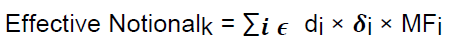
Effective notional for each maturity category = Σ(trade-level adjusted notional × supervisory delta × maturity factor), with full offsetting for each of the three maturity categories, in each hedging set (that is, same currency)2. Apply Supervisory Factors Add-on for each maturity category in a hedging set (that is, same currency) = Effective Notional Amount for maturity category × interest rate supervisory factor 3. Apply Supervisory Correlations Add-on for each hedging set = Σ(Add-ons for maturity categories), aggregating across maturity categories for a hedging set. One hedging set for each currency. 4. Aggregate Simple summation of the add-ons for the different hedging sets Calculate Effective Notional Amount
The adjusted notional of each trade is calculated by multiplying the notional amount by the calculated supervisory duration SD as defined in the Standards.
d = Trade Notional × SD = Trade Notional × (exp(-0.05×S) – exp(-0.05 × E)) / 0.05
Trade Notional Amount Time Bucket S E Supervisory Duration SD Adjusted Notional d Trade 1 10,000,000 3 0 10 7.869386806 78,693,868.06 Trade 2 10,000,000 2 0 4 3.625384938 36,253,849.38 Trade 3 5,000,000 3 1 11 7.485592282 37,427,961.41 Calculate Maturity Category Effective Notional
A supervisory delta is assigned to each trade in accordance with the Standards. In particular:
- •Trade 1 is long in the primary risk factor (the reference floating rate) and is not an option so the supervisory delta is equal to 1.
- •Trade 2 is short in the primary risk factor and is not an option; thus, the supervisory delta is equal to -1.
- •Trade 3 is an option to enter into an interest rate swap that is short in the primary risk factor and therefore is treated as a purchased put option. As such, the supervisory delta is determined by applying the relevant formula using 50% as the supervisory option volatility and 1 (year) as the option exercise date. Assume that the underlying price (the appropriate forward swap rate) is 6% and the strike price (the swaption’s fixed rate) is 5%.
The trade-level supervisory delta is therefore:
Trade Delta Instrument Type Trade 1 1 linear, long (forward and swap) Trade 2 -1 linear, short (forward and swap) Trade 3 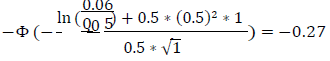
purchased put option The Maturity Factor MF is 1 for all the trades since they are un-margined and have remaining maturities in excess of one year.
Based on the maturity categories, the Effective Notional D for the USE and EUR hedging sets at the level of the maturity categories are as shown in the table below:
Hedging Set Time Bucket Adjusted Notional Supervisory Delta Maturity Factor Maturity category-level Effective Notional D HS 1 (USD) 3 78,693,868 1 1 78,693,868 2 36,253,849 -1 1 -36,253,849 HS 2 (EUR) 3 37,427,961 -0.27 1 -10,105,550 In particular:
Hedging set USD, time bucket 3: D = 1 * 78,693,868 * 1 = 78,693,868
Hedging set USD, time bucket 2: D = -1 * 36,253,849 * 1 = -36,253,849
Hedging set EUR, time bucket 3: D = -0.27 * 37,427,961 * 1 = -10,105,550
Apply Supervisory Factor
The add-on must be calculated for each hedging set.
For the USD hedging set there is partial offset between the two USD trades:
Effective notional(IR) USD = [D22 + D32 + 1.4 x D2 x D3]1/2
= [(-36,253,849)2 + 78,693,8682 + 1.4 × (-36,253,849) × 78,693,868]1/2
= 59,269,963
For the Hedging set EUR there is only one trade (and one maturity category):
Effective notional(IR)EUR = 10,105,550
In summary:
Hedging set Time Bucket Maturity category-level Effective Notional Dj,k Hedging Set level Effective Notional Dj,k (IR) HS 1 (USD) 3 78,693,868 59,269,963
(Partial offset)2 -36,253,849 HS 2 (EUR) 3 -10,105,550 10,105,549.58 Aggregation of the calculated add-ons across different hedging sets:
Effective Notional(IR) = 59,269,963 + 10,105,550 = 69,375,513 (No offset between hedging sets) The asset class is interest rates; thus the applicable Supervisory factor is 0.50%. As a result:
Add-on = SF × Effective Notional = 0.005 × 69,375,513 = 346,878
Supervisory Correlation Parameters
Correlation is not applicable to the interest rate asset class, and there is no other asset class in the netting set in this example.
Add-on Aggregation
For this netting set, the interest rate add-on is also the aggregate add-on because there are no trades assigned to other asset classes. Thus, the aggregate add-on = 346,878
Multiplier
The multiplier is given by:
multiplier = min { 1; Floor+(1-Floor) × exp [(V-C) /(2 ×(1-Floor)×Add-onagg)]}
= min {1; 0.05 + 0.95 × exp [60,000 / (2 × 0.95 × 346,878]}
=1
Final Calculation of PFE
In this case the multiplier is equal to one, so the PFE is the same as the aggregate Add-On:
PFE = multiplier × Add-onagg = 1 × 346,878 = 346,878
3. EAD Calculation
The exposure EAD to be risk weighted for counterparty credit risk capital requirements purposes is therefore
EAD = 1.4 * (RC + PFE) = 1.4 x (60,000 + 346,878) = 569,629
B. Illustration 2
Consider a netting set with three credit derivatives: one long single-name CDS written on Firm A (rated AA), one short single-name CDS written on Firm B (rated BBB), and one long CDS index (investment grade). All notional amounts and market values are denominated in USD. This netting set is not subject to a margin agreement and there is no exchange of collateral (independent amount/initial margin) at inception. The table below summarizes the relevant contractual terms of the three derivatives.
Trade # Nature Reference entity / index name Rating reference entity Residual maturity Base currency Notional (thousands) Position Market value (thousands) 1 Single-name CDS Firm A AA 3 years USD 10,000 Protection buyer 20 2 Single-name CDS Firm B BBB 6 years EUR 10,000 Protection seller -40 3 CDS index CD X.IG Investment grade 5 years USD 10,000 Protection buyer 0 According to the Standards, the EAD for un-margined netting sets is given by:
EAD = 1.4 * (RC + PFE)
1. Replacement Cost Calculation
The replacement cost is calculated at the netting set level as a simple algebraic sum (floored at zero) of the derivatives’ market values at the reference date. Thus, using the market values indicated in the table (expressed in thousands):
RC = max {V - C; 0} = max {20 - 40 + 0; 0} = 0
Since V-C is negative (i.e. -20,000), the multiplier will be activated (i.e. it will be less than 1). Before calculating its value, the aggregate add-on needs to be determined.
2. Potential Future Exposure Calculation
The following table illustrates the steps typically followed for the add-on calculation:
Steps Activities 1. Calculate Effective Notional Calculate supervisory duration
Calculate trade-level adjusted notional = trade notional (in domestic currency) × supervisory duration
Calculate trade-level effective notional amount = trade-level adjusted notional × supervisory delta × maturity factor
Calculate effective notional amount for each entity by summing the trade-level effective notional amounts for all trades referencing the same entity (either a single entity or an index) with full offsetting2. Apply Supervisory Factors Add-on for each entity in a hedging set = Entity-level Effective Notional Amount × Supervisory Factor, which depends on entity’s credit rating (or investment/speculative for index entities) 3. Apply Supervisory Correlations Entity-level add-ons are divided into systematic and idiosyncratic components weighted by the correlation factor 4. Aggregate Aggregation of entity-level add-ons with full offsetting in the systematic component and no offsetting in the idiosyncratic component Effective Notional Amount
The adjusted notional of each trade is calculated by multiplying the notional amount with the calculated supervisory duration SD specified in the Standards.
d= Trade Notional × SD = Trade Notional × {exp(-0.05×S) – exp(-0.05 × E)} / 0.05
Trade Notional Amount S E Supervisory Duration SD Adjusted Notional d Trade 1 10,000,000 0 3 2.785840471 27,858,405 Trade 2 10,000,000 0 6 5.183635586 51,836,356 Trade 3 10,000,000 0 5 4.423984339 44,239,843 The appropriate supervisory delta must be assigned to each trade: in particular, since Trade 1 and Trade 3 are long in the primary risk factor (CDS spread), their delta is 1; in contrast, the supervisory delta for Trade 2 is -1.
Trade Delta Instrument Type Trade 1 1 linear, long (forward and swap) Trade 2 -1 linear, short (forward and swap) Trade 3 1 linear, long (forward and swap) Thus, the entity-level effective notional is equal to the adjusted notional times the supervisory delta times the maturity factor (where the maturity factor is 1 for all three derivatives).
Trade Adjusted Notional Supervisory Delta Maturity Factor Entity Level Effective Notional Trade 1 27,858,405 1 1 27,858,405 Trade 2 51,836,356 -1 1 -51,836,356 Trade 3 44,239,843 1 1 44,239,843 Supervisory Factor
The add-on must now be calculated for each entity. Note that all derivatives refer to different entities (single names/indices). A supervisory factor is assigned to each single-name entity based on the rating of the reference entity, as specified in Table 1 in the relevant Standards. This means assigning a supervisory factor of 0.38% for AA-rated firms (Trade 1) and 0.54% for BBB-rated firms (for Trade 2). For CDS indices (Trade 3), the supervisory factor is assigned according to whether the index is investment or speculative grade; in this example, its value is 0.38% since the index is investment grade.
Asset Class Subclass ρ SF Credit, Single Name AA 50% 0.38% Credit, Single Name BBB 50% 0.54% Credit, Index IG 80% 0.38% Thus, the entity level add-ons are as follows:
Add-on(Entity) = SF × Effective Notional
Trade Effective Notional Supervisory factor SF Add-on (Entity) Trade 1 27,858,405 0.38% 105,862 Trade 2 -51,836,356 0.54% -279,916 Trade 3 44,239,843 0.38% 168,111 Supervisory Correlation Parameters
The add-on calculation separates the entity level add-ons into systematic and idiosyncratic components, which are combined through weighting by the correlation factor. The correlation parameter ρ is equal to 0.5 for the single-name entities (Trade 1-Firm A and Trade 2-Firm B) and 0.8 for the index (Trade 3-CDX.IG) in accordance with the requirements of the Standards.
Add-on(Credit) = [ [ ∑k ρk CR × Add-on (Entityk) ]2 + ∑k (1- (ρk CR)2) × (Add-on (Entityk))2]1/2
Trade ρ Add-on(Entityk) ρ × Add-on(Entityk) (1 – ρ2) (1 – ρ2) × (Add-on(Entityk))2 Trade 1 50% 105,862 52,931 0.75 8,405,062,425 Trade 2 50% -279,916 -139,958 0.75 58,764,860,350 Trade 3 80 % 168,111 134,489 0.36 10,174,120,000 Systematic Component 47,462 Idiosyncratic Component 77,344,042,776 Full offsetting No offsetting Add-on Aggregation
For this netting set, the interest rate add-on is also the aggregate add-on because there are no trades assigned to other asset classes. Thus, the aggregate add-on = 346,878
Aggregation of entity-level add-ons with full offsetting in the systematic component and no offsetting benefit in the idiosyncratic component.
Systematic Component 47,462 Idiosyncratic Component 77,344,042,776 Thus,
Add-on = [ (47,462)2 + 77,344,042,776 ]1/2 = 282,129
Multiplier
The multiplier is given by
multiplier = min {1; Floor+(1-Floor) × exp [(V-C)/(2×(1-Floor)×Add-onagg)]}
= min {1; 0.05 + 0.95 × exp [-20,000 / (2 × 0.95 × 282,129)]}
=0.96521
Final Calculation of PFE
PFE = multiplier × Add-onagg = 0.96521 × 282,129= 272,313
3. EAD Calculation
The exposure that would be risk-weighted for the purpose of counterparty credit risk capital requirements is therefore:
EAD = 1.4 * (RC + PFE) = 1.4 x (0 + 272,313) = 381,238
C. Illustration 3
Consider a netting set with three commodity forward contracts. All notional amounts and market values are denominated in USD. This netting set is not subject to a margin agreement and there is no exchange of collateral (independent amount/initial margin) at inception. The table below summarizes the relevant contractual terms of the three commodity derivatives.
Trade # Nature Underlying Position Direction Residual maturity Notional (thousands) Market value (thousands) 1 Forward (WTI)
Crude OilProtection Buyer Long 9 months 10,000 -50 2 Forward (Brent)
Crude OilProtection Seller Short 2 years 20,000 -30 3 Forward Silver Protection Buyer Long 5 years 10,000 100 1. Replacement Cost Calculation
The replacement cost is calculated at the netting set level as a simple algebraic sum (floored at zero) of the derivatives’ market values at the reference date, provided that value is positive. Thus, using the market values indicated in the table (expressed in thousands):
RC = max {V - C; 0} = max {100 - 30 - 50; 0} = 20
The replacement cost is positive and there is no exchange of collateral (so the bank has not received excess collateral), which means the multiplier will be equal to 1.
2. Potential Future Exposure Calculation
The following table illustrates the steps typically followed for the add-on calculation, for each of the four commodity hedging sets with non-zero exposure:
Steps Activities 1. Calculate Effective Notional Calculate trade-level adjusted notional = current price × number of units referenced by derivative
Calculate trade-level effective notional amount = trade-level adjusted notional × supervisory delta × maturity factor
Calculate effective notional for each commodity-type = Σ(trade-level effective notional) for trades referencing the same commodity type, with full offsetting in commodity type2. Apply Supervisory Factors Add-on for each commodity type in a hedging set = Commodity-type Effective Notional Amount × Supervisory Factor 3. Apply Supervisory Correlations Commodity-type add-ons are divided into systematic and idiosyncratic components weighted by the correlation factor 4. Aggregate Aggregation of commodity-type add-ons with full offsetting in the systematic component and no offsetting in the idiosyncratic component
Simple summation of absolute values of add-ons across the four hedging setsEffective Notional Amount
Trade-level Adjusted Notional calculation for each commodity derivative trade:
di(COM) = current price per unit × number of units in the trade
Trade Current price per unit (unit is barrel for oil; ounces for silver) Number of units in the trade Adjusted Notional Trade 1 100 100 barrels 10,000 Trade 2 100 200 barrels 20,000 Trade 3 20 500 ounces 10,000 The appropriate supervisory delta must be assigned to each trade:
Trade Delta Instrument Type Trade 1 1 linear, long (forward & swap) Trade 2 -1 linear, short (forward & swap) Trade 3 1 linear, long (forward & swap) Since the remaining maturity of Trade 1 is less than a year, at nine months (approximately 187 business days), and the trade is un-margined, its maturity factor is scaled down by the square root of 187/250 in accordance with the requirements of the Standards. On the other hand, the maturity factor is 1 for Trade 2 and for Trade 3, since the remaining maturity of those two trades is greater than one year and they are un-margined.
The trade-level effective notional is equal to the adjusted notional times the supervisory delta times the maturity factor. The basic difference between the WTI and Brent forward contracts effectively is ignored since they belong to the same commodity type, namely “Crude Oil” within the “Energy” hedging set, thus allowing for full offsetting. (In contrast, if one of the two forward contracts were on a different commodity type within the “Energy” hedging set, such as natural gas, with the other on crude oil, then only partial offsetting would have been allowed between the two trades.) Therefore, Trade 1 and Trade 2 can be aggregated into a single effective notional, taking into account each trade’s supervisory delta and maturity factor.

Hedging Set Commodity Type Trade Adjusted Notional Supervisory Delta Maturity Factor Effective Notional Energy Crude Oil Trade 1 10,000 1 10,000 x 1 x 0.865 + 20,000x(-1)x1 =-11,350 (full off-setting within the ‘Crude Oil’ commodity type) Energy Crude Oil Trade 2 20,000 -1 1 Metals Silver Trade 3 10,000 1 1 10,000 Supervisory Factor
For each commodity-type in a hedging set, the effective notional amount must be multiplied by the correct Supervisory Factor (SF). As described in the Standards, the Supervisory Factor for both the Crude Oil commodity type in the Energy hedging set and the Silver commodity type in the Metals hedging set is SF=18%.
Thus, the add-on by hedging set and commodity type is as follows:
Add-on(Typekj) = SFTypek(Com) × Effective NotionalTypek(Com)
Hedging Set Commodity Type Effective Notional Supervisory Factor SF Add-on by HS and Commodity type Energy Crude Oil -11,350 18% -2,043 Metals Silver 10,000 18% 1,800 Supervisory Correlation Parameters
The commodity-type add-ons in a hedging set are decomposed into systematic and idiosyncratic components. The commodity subclass correlations parameters are as stated in the Standards, in this case 40% for commodities.
Thus, the hedging set level add-ons are calculated for each commodity hedging set:
Add-on(COM) = [( Σk ρj(COM) × Add-on (Typekj) )2 + Σk (1- (ρj(COM) )2) × (Add-on (Type j))2]k1/2
Hedging Set Commodity Type ρ Add-on(Typek) Systematic Component (ρ × Add-on(Typek))2 (1 – ρ2) Idiosyncratic Component (1 – ρ2) x (Add-on(Typek)) 2 Add-onj (Only one commodity type in each HS) Energy Crude Oil 40% -2,043 (-817)2 0.84 0.84 × (-2,043)2 2,043 Metals Silver 40% 1,800 (720)2 0.84 0.84 × (1,800)2 1,800 However, in this example, since only one commodity type within the “Energy” hedging set is populated (i.e. all other commodity types within that hedging set have a zero add-on), the resulting add-on for the hedging set is the same as the add-on for the commodity type. This calculation shows that when there is only one commodity type within a commodity hedging set, the hedging-set add-on is equal to the absolute value of the commodity-type add-on. (The same comment applies to the commodity type “Silver” in the “Metals” hedging set.)
Add-on Aggregation
Aggregation of commodity-type add-ons uses full offsetting in the systematic component and no offsetting benefit in the idiosyncratic component in each hedging set. As noted earlier, in this example there is only one commodity type per hedging set, which means no offsetting benefits. Computing the simple summation of absolute values of add-ons for the hedging sets:
Add-on = Σj Add-onj
Add-On = 2,043 + 1,800 = 3,843
Multiplier
The multiplier is given by
multiplier = min {1; Floor+(1-Floor) × exp [(V-C)/(2×(1-Floor)×Add-onagg)]}
= min {1; 0.05 + 0.95 × exp [20 / (2 × 0.95 × 3,843)]}
= 1, since V-C is positive.
Final Calculation of PFE
PFE = multiplier × Add-onagg = 1 × 3,843 = 3,843
3. EAD Calculation
The exposure EAD to be risk weighted for counterparty credit risk capital requirements purposes is therefore
EAD = 1.4 * (RC + PFE) = 1.4 x (20 + 3,843) = 5,408